
One the downsides to having all kinds of templates and style sheets in MS Excel is that you pretty much get locked in to creating sheets that look like everyone else’s; which doesn’t do much for creativity or inspirational ideas. This is why it’s a good idea to learn how to use Excels formatting tools.
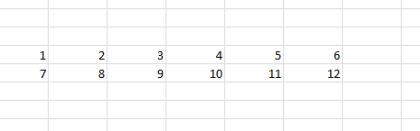
To begin, start by creating a table that has some rows and tables, like this:
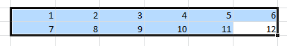
Then, highlight the whole thing…
Next, click on it with your right mouse button, to get this popup men:
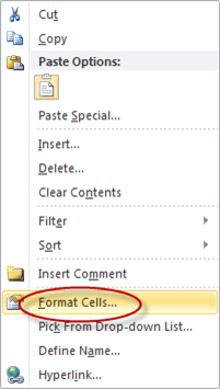
Choose the Format Cells option, to get this little window:
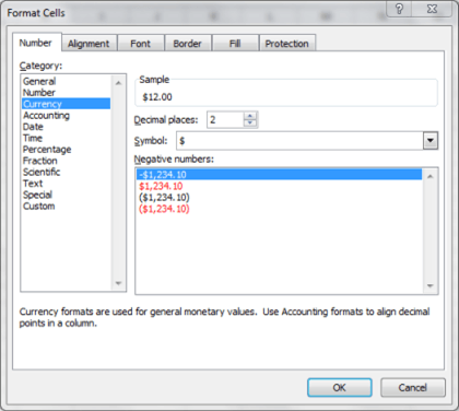
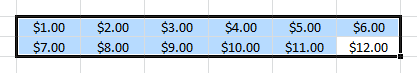
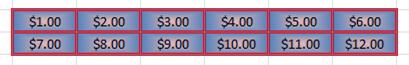
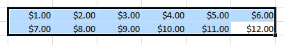
Using just these simple tools, you can create pretty much anything you’ve seen in Excel’s pre-formatted templates. To see how, we’ll move right across the top menu bar, first up, is the Number format option list, here we can set the number in our table to represent a regular number, a dollar amount, a time or date, or whatever we like; for this example, we’ll chose currency and go with the default of two decimal places, that makes out table look like this:

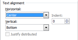
Next on the menu is Alignment:
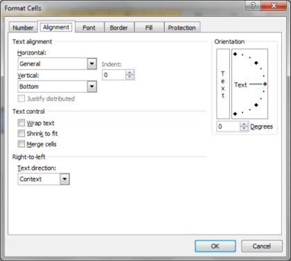
All of these options are about making the contents of a cell or group of cells sit in their cell the way you want. Mostly they are about putting cell content at the cell, top, bottom, left right or centered; or whether text is wrapped on not; there is also an option to make text or numbers appear at an angle in the cell; but because we just want to show currency, we’ll chose to center it and that’s all:

Which makes our table looks like this:
Next on the menu is Font:

Since it works exactly like the Font command in every other Windows application we’ll just stick with the default and move on to the Border option:
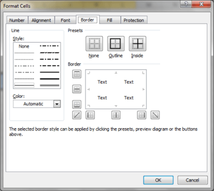
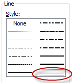
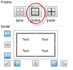
This is the section where a lot of the magic happens, it’s divided into three sections; Line, Presets, and Color. The line section lets you choose what sort of border to draw around whatever cells you’ve highlighted, In this case, we’ll choose a double bar:
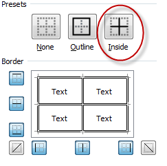
You’ll notice that nothing happens when you choose it, and that’s because you have to tell Excel where you want that border to exist, and that’s what the Presets section is about. Since we want a border that goes all the way around the outside of our highlighted area, we choose this one:

But, we’d also like all the borders between each cell to have a border as well, so we choose this option too:
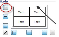
The other little icons are for adding or removing certain walls of the border, like say if you’d like to not have a border across the top, you’d click on this one:
Then, all that’s left to do is choose a color for our border:
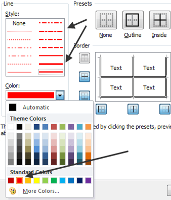
Notice how once you pick a color, the line color above changes to reflect your choice. Unfortunately, the border you added earlier does not change, so you make your choices again to make them the new color you’ve chosen.
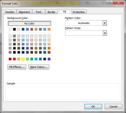
Next up on the menu is the Fill feature:
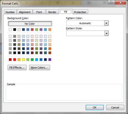
Here you can add color to the background of the cells themselves. You have two options, to fill the cells you’ve highlighted with a background color or a pattern with a color. We’ll look at background first.
You can simply click on a color to choose a background color, or or click the More Colors button for a color wheel that gives you more color options, or you can click on the Fill Effects button to get this:
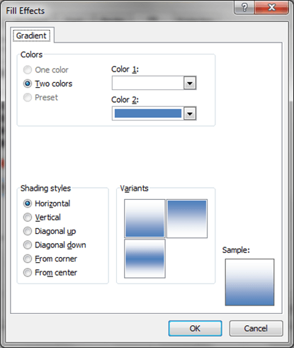
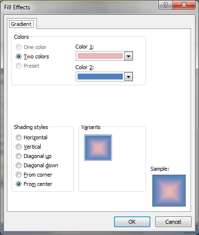
Here you can add colors or a shading style to create a gradient (a gradient is where color changes slowly across a cell or cells). The top part of the pane allows you to choose one or two colors of your choice, while the bottom selects the direction of the gradient. For our example, we’re going to choose light pink and a somewhat dark blue for the colors and from center as our shading style:
Then click the OK button and we’re about done.
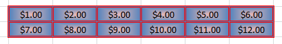
The last menu choice Protection, isn’t really a formatting option, it allows you to lock the contents of cells so that you don’t accidently overwrite formulas and such. For now, let’s just click the OK button and take a look at what we’ve done to our original table:
The effects shown here can be used in very nearly unlimited and creative ways to show off your sheets in ways that stand out far more than you’ll ever get using the cookie-cuter styles that come with Excel.
They can be used in titles, or in descriptions or to create extra borders around the edges of your sheet, or to highlight certain areas, etc. They can also be used to alter your sheet after applying a style if you’d like to change things up just a little bit.
To begin, start by creating a table that has some rows and tables, like this:

Then, highlight the whole thing…

Next, click on it with your right mouse button, to get this popup men:

Choose the Format Cells option, to get this little window:
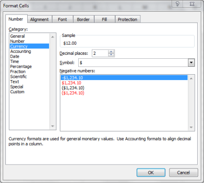
Using just these simple tools, you can create pretty much anything you’ve seen in Excel’s pre-formatted templates. To see how, we’ll move right across the top menu bar, first up, is the Number format option list, here we can set the number in our table to represent a regular number, a dollar amount, a time or date, or whatever we like; for this example, we’ll chose currency and go with the default of two decimal places, that makes out table look like this:
Next on the menu is Alignment:

All of these options are about making the contents of a cell or group of cells sit in their cell the way you want. Mostly they are about putting cell content at the cell, top, bottom, left right or centered; or whether text is wrapped on not; there is also an option to make text or numbers appear at an angle in the cell; but because we just want to show currency, we’ll chose to center it and that’s all:
Which makes our table looks like this:

Next on the menu is Font:
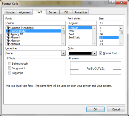
Since it works exactly like the Font command in every other Windows application we’ll just stick with the default and move on to the Border option:
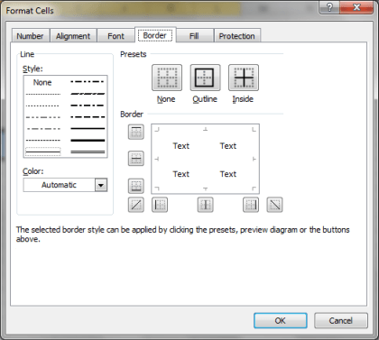
This is the section where a lot of the magic happens, it’s divided into three sections; Line, Presets, and Color. The line section lets you choose what sort of border to draw around whatever cells you’ve highlighted, In this case, we’ll choose a double bar:

You’ll notice that nothing happens when you choose it, and that’s because you have to tell Excel where you want that border to exist, and that’s what the Presets section is about. Since we want a border that goes all the way around the outside of our highlighted area, we choose this one:
But, we’d also like all the borders between each cell to have a border as well, so we choose this option too:

The other little icons are for adding or removing certain walls of the border, like say if you’d like to not have a border across the top, you’d click on this one:

Then, all that’s left to do is choose a color for our border:

Notice how once you pick a color, the line color above changes to reflect your choice. Unfortunately, the border you added earlier does not change, so you make your choices again to make them the new color you’ve chosen.
Next up on the menu is the Fill feature:
Here you can add color to the background of the cells themselves. You have two options, to fill the cells you’ve highlighted with a background color or a pattern with a color. We’ll look at background first.
You can simply click on a color to choose a background color, or or click the More Colors button for a color wheel that gives you more color options, or you can click on the Fill Effects button to get this:

Here you can add colors or a shading style to create a gradient (a gradient is where color changes slowly across a cell or cells). The top part of the pane allows you to choose one or two colors of your choice, while the bottom selects the direction of the gradient. For our example, we’re going to choose light pink and a somewhat dark blue for the colors and from center as our shading style:

Then click the OK button and we’re about done.
The last menu choice Protection, isn’t really a formatting option, it allows you to lock the contents of cells so that you don’t accidently overwrite formulas and such. For now, let’s just click the OK button and take a look at what we’ve done to our original table:
The effects shown here can be used in very nearly unlimited and creative ways to show off your sheets in ways that stand out far more than you’ll ever get using the cookie-cuter styles that come with Excel.
They can be used in titles, or in descriptions or to create extra borders around the edges of your sheet, or to highlight certain areas, etc. They can also be used to alter your sheet after applying a style if you’d like to change things up just a little bit.
No comments:
Post a Comment